Which indoor system can carry your building’s demand?

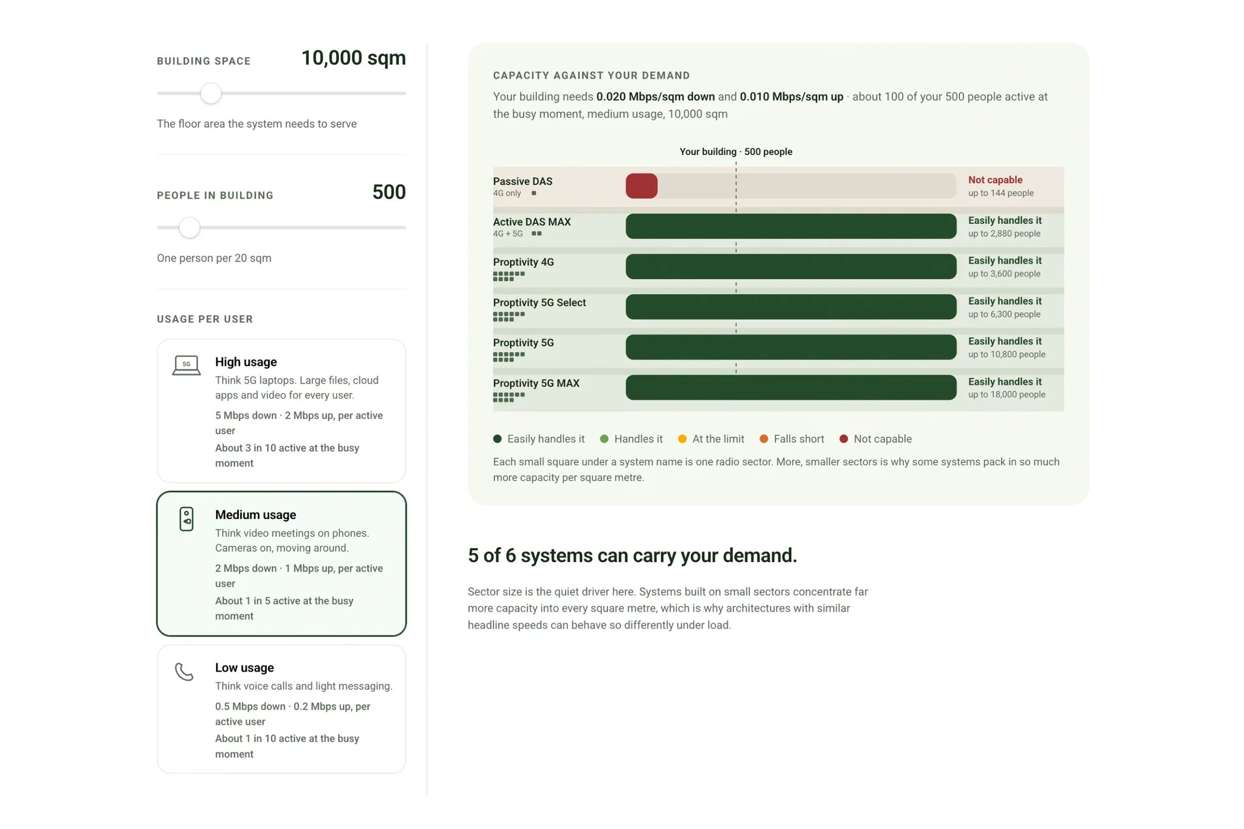
All scenarios assume three mobile operators, each with 100 MHz of 5G spectrum (3.5 GHz band) and 20 MHz of LTE spectrum. Each system’s peak throughput per cell is derived from its radio configuration, reduced by an efficiency factor and any distribution overhead, multiplied by three operators, then divided by the cell’s coverage area to give a capacity density in Mbps per square metre, downlink and uplink separately. A system’s verdict is set by whichever direction is the tighter constraint.

Where the peak rates come from:

The 4G figure assumes a modern radio with 256QAM: 20 MHz with two spatial streams peaks around 200 Mbps, and a single stream around 100 Mbps. The 5G figures follow the same logic on 100 MHz of TDD spectrum: roughly 800 Mbps with two streams and 1600 Mbps with four. The 5G Select tier runs 5G on re-farmed 4G frequencies in the mid and low bands, where far less spectrum is available, which is why its 5G layer peaks around 300 Mbps rather than 800. Uplink shares follow from how each technology divides its resources: FDD 4G has a dedicated uplink carrier (about 40% of downlink in practice), while TDD 5G shares one band between directions with a frame pattern that allocates roughly a fifth of capacity to uplink. The same 20% is applied to all 5G layers regardless of architecture.

System assumptions:

• Passive DAS (4G only): a passive coax network cannot carry multiple MIMO streams and handles the 3.5 GHz 5G band poorly over distance, so it is modelled as single-stream 4G only: 100 Mbps DL max, 60% efficiency, 20% overhead for coax losses; UL 40% of DL. Cell size 20,000 sqm, typical for as-deployed passive systems.
• Active DAS MAX (4G + 5G): 4G 2×2 MIMO at 200 Mbps plus 5G 4×4 MIMO at 1600 Mbps, both at 60% efficiency with a 20% overhead for the RF chain and signal conversion stages; UL 40% of DL for 4G and 20% for 5G. Cell size 10,000 sqm, typical for as-deployed active DAS, where one cell usually spans several floors to contain head-end cost.
• Proptivity 4G: 4G 2×2 MIMO, 200 Mbps DL max, 60% efficiency; UL 40% of DL. Cell size 2,000 sqm.
• Proptivity 5G Select: 4G as above, plus 5G on re-farmed 4G frequencies, 2×2 MIMO, 300 Mbps DL max, 60% efficiency; UL 20% of DL. Cell size 2,000 sqm.
• Proptivity 5G: 4G as above, plus full-band 5G, 2×2 MIMO, 800 Mbps DL max, 60% efficiency; UL 20% of DL. Cell size 2,000 sqm.
• Proptivity 5G MAX: 4G as above, plus full-band 5G, 4×4 MIMO, 1600 Mbps DL max, 60% efficiency; UL 20% of DL. Cell size 2,000 sqm.

Cell sizes reflect typical as-deployed configurations rather than physical limits. Any architecture can in principle be sectorised more densely, but cost structure drives the sizes above in practice, and cell size is the single strongest driver of capacity per square metre: halving the cell area doubles the capacity density before any radio improvement is counted.

Worked example, Proptivity 5G MAX:

5G layer: 1600 Mbps x 60% = 960 Mbps DL, and 20% of that is 192 Mbps UL. 4G layer: 200 Mbps x 60% = 120 Mbps DL and 48 Mbps UL. Per operator that totals 1,080 Mbps DL and 240 Mbps UL. Across three operators: 3,240 Mbps DL and 720 Mbps UL per cell. Over a 2,000 sqm cell: 3,240 / 2,000 = 1.62 Mbps/sqm DL and 720 / 2,000 = 0.36 Mbps/sqm UL. Every system in the table below is computed the same way.

Resulting capacity density (3 operators):

Usage profiles and busy-moment activity:

Not everyone in a building consumes capacity at the same instant, so demand is dimensioned for the busy moment rather than for the full headcount, the same principle traditional voice networks were planned on. Each profile therefore carries an assumed share of people active simultaneously: 1 in 10 for voice-style use, 1 in 5 for video-heavy phone use, and 3 in 10 for laptop-grade work. Building demand is then: people in building x active share x per-active-user rate / floor area, giving a demand density in Mbps/sqm for each direction that is compared against each system’s capacity density. The “up to N people” figures in the chart use the same logic in reverse.

Verdict thresholds:

Utilisation is your demand divided by the system’s capacity, taking the worse of downlink and uplink. Up to 60% utilisation is shown as easily handled, up to 85% as handled, up to 100% as at the limit, up to 130% as falling short, and above that as not capable.

Simplifications:

• Demand is assumed to be evenly spread across the space; real buildings concentrate users in hotspots such as meeting floors and atriums.
• Peak rates assume good radio conditions throughout the cell and 256QAM-capable devices; edge-of-cell users achieve less.
• The busy-moment activity shares are planning assumptions; an unusual event such as a full-house town hall meeting can push activity well above them for short periods.
• The voice profile is set generously at 0.5 Mbps down; actual voice calls use less, so the allowance also covers signalling and background app traffic.